Copyright ©2019 Thomas Schwengler. A significantly updated and completed 2019 Edition is available.

Chapter 3
Radio Propagation Modeling

Before studying details of propagation we need to define a few notation conventions, which will require the reader to be familiar with the following general concepts of electromagnetic field and wave theory.

• Wireless communications signals of interest are electromagnetic waves, and may be derived in free space from the electric field .
• The power density of the electromagnetic wave may be written in the form of the Poynting vector: = ×. The power density is the modulus of the Poynting vector P_d = ||.
• In free space the electric and magnetic field strength are related by || = η₀||, and the power density of the electromagnetic wave is proportional to the modulus squared of the electric field: P_d = |E|²∕η₀, where η₀ ≈ 377 Ω is the impedance of the vacuum (and by approximation of air). ²
• The electric field may be identified with the transmitted signal S(t) = s(t) ⋅ exp(j2πft), where s(t) is the (real) user encoded information to transmit, and f is the carrier frequency. S(t) is a complex function which real part Re{S(t)} = s(t)⋅cos(2πft) is the physical quantity of interest; although the complex function S(t) is usually used for simpler mathematical treatment, one should remember that its real part is the meaningful quantity. ³
• Similarly, we identify the received signal with the received electric field; we denote the received signal: R(t) = r(t) ⋅ exp(j2πft).
• Given the above, received power densities are given by the expression P_d(t) = |R(t)|²∕η₀.
• Actual received power P_r also depends on the effective area of the receiving antenna P_r(t) = A_eP_d(t) = A_e|R(t)|²∕η₀ (see further details in §3.2).

Some details of E-field propagation will be studied later with ray tracing; but most of the remainder of the section deals with very simple expressions of power levels for paths loss modeling.

3.1 Propagation Characteristics

Between transmitter and receiver, the wireless channel is modeled by several key parameters. These parameters vary significantly with the environment, they are often separated in three types [1] [3]:

Distance Dependence

of path loss (measured in dB) is approximated by L(d) = L₀ +10n×log(d∕d₀), where n is the path loss exponent, which varies with terrain and environment, and L₀ and d₀ are parameters described further in §3.3 and §3.4.

Large-scale Shadowing

causes variations over larger areas, and is caused by terrain, building, and foliage obstructions; its impact on link budgets is detailed further in §4.1.

The large-scale fading due to various obstacles is commonly accepted to follow a log-normal distribution ([17], [18], [19] ch. 7). This means that its attenuation x measured in dB is normally distributed N(m,σ), with mean m, standard deviation σ, and which probability density function is given by the usual Gaussian formula:

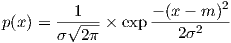(3.1)

Small-scale fading

causes great variation within a half wavelength. It is caused by multipath and moving scatterers, and is detailed further in §??. Resulting fades are usually approximated by Rayleigh, Ricean, or similar fading statistics – measurements also show good fit to Nakagami-m and Weibull distributions.

Radio systems rely on diversity, equalizing, channel coding, and interleaving schemes to mitigate its impact.

Copyright ©2019 Thomas Schwengler. Significantly updated and completed in 2019 Edition available here.

Different spectrum bands have very different propagation characteristics and require different prediction models. Some propagation models are well suited for computer simulation in presence of detailed terrain and building data; others aim at providing simpler general path loss estimates [20].

3.2 Free-Space Propagation

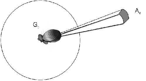
A simple approach to propagation modeling is to estimate the power ratio between transmitter and receiver as a function of the separation distance d, that ratio is referred to as path loss. A physical argument of conservation of energy leads to the Friis’ power transmission formula in free space. A transmitted power source P_t radiates spherically, with an antenna gain G_t; the portion of that power impinging an effective area A_e at a distance d is P_r = P_tG_tA_e∕(4πd²). The effective area of an antenna is related to antenna gain by A_e∕λ² = G_r∕4π, which is used here for the receiving antenna (of gain G_r), and thus yields:

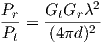(3.2)

(P_t and P_r are the transmitted and received power, G_t and G_r are the transmitter and receiver antenna gain, λ is the wavelength of the signal, and d is the separation distance).

This equation shows a free-space dependence in 1∕d², and is often expressed in decibels (dB): L(dB) = 10 × log .

In many cases, antenna gains are considered separately, and one choses to focus on the path loss between the two antennas. The path loss reflects how much power is dissipated between transceiver and receiver antennas (without counting any antenna gain). The path loss variation with distance is d², or 20 log(d) in dB, which is characteristic of a free space model. The exponent (here n = 2) is called the path loss exponent, and its value varies with models. Path loss is often expressed as a function of frequency (f), distance (d), and a scaling constant that contains all other factors of the formula. For instance:

(3.3)

where f₀ = 1 MHz, and d₀ = 1 km. These reference values are arbitrary and chosen to be convenient to use values in MHz and km in the formula.

Note that the constant 32.45 changes if the reference frequency f₀ and the reference distance d₀ are chosen to be different. Many presentations will refer to the formula as L(dB) = 32.45 + 20 × log(f) + 20 × log(d), adding a statement such as “f is in MHz and d is in km”. That shorter notation is equivalent to equation (3.3), but should be treated carefully: with the loss of f₀ and d₀ in the equation, mistakes can be introduced by further manipulating the expression.

3.3 Ray Tracing

Ray tracing is a method that uses a geometric approach, and examines what paths the wireless radio signal takes from transmitter to receiver as if each path was a ray of light (reflecting off surfaces). Ray-tracing predictions are good when detailed information of the area is available. But the predicted results may not be applicable to other locations, thus making these models site-specific.

Nevertheless, fairly general models may be devised from ray tracing concepts. The well-known two-ray model uses the fact that for most wireless propagation cases, two paths exist from transmitter to receiver: a direct path and a bounce off the ground. That model alone shows some important variations of the received signal with distance. [1] [3] Ray tracing models are extensively used in software propagation prediction packages, which justifies a closer look at them in this section.

3.3.1 Ray Tracing Notations

Rays are an optical approximation of the electromagnetic wave; as seen earlier, in free space it is convenient to focus on the propagation of the electric field. The (complex) transmitted electric field is noted S(t), the received field is R(t), we define the ratio p₀(t) = R(t)∕S(t). Then the power link budget between transmitter and receiver can be written P_r∕P_t = |p₀|².

In the next few subsections, we will consider how the electric field propagates, and we will compute various expressions for p₀(t) in various conditions; each time the final step will be to take its modulus squared in order to derive the path loss.

3.3.2 Two-Ray Model

With these few notation conventions we can derive a simple but useful model with two rays.

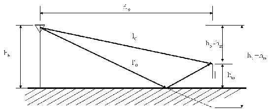
Figure 3.2 shows a fixed tower (e.g. in a cellular system) at a height h_b, and a client device at a distance d₀, and at a height h_m (usually lower). The figure shows a direct ray and an indirect ray bouncing off the ground, assumed to be a perfect plane (this assumption is referred to as the flat-earth model). ⁴

It is easy to see from this figure that the two path lengths are:

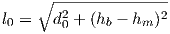(3.4)

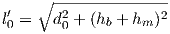(3.5)

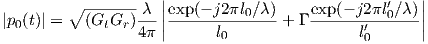
The received signal at a distance d₀ is therefore:

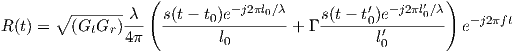(3.6)

where λ = c∕f is the wavelength, t₀ = l₀∕c (respectively t′₀ - l′₀∕c) is the time needed for the wave to propagate over distance l₀ (respectively l′₀), and Γ is the ground reflection coefficient. For now let us simply assume perfect reflection and use Γ = -1; will elaborate further on Γ in §3.3.3. ⁵

Another important assumption must be made here to simplify the model: we will assume that propagation time differences are small compared to the symbol length of the useful information, that is s(t-t₀) = s(t-t′₀). For a bounce off the ground, that assumption is fairly safe, but in general we will have to recall that such an assumption means that we assume that the delay spread is small compared to transmitted symbol rates.

So we obtain:

(3.7)

which simplifies for distances much greater than heights (d₀ ≈ l₀ ≈ l′₀):

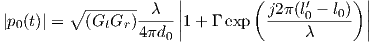(3.8)

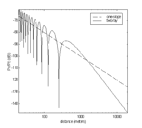
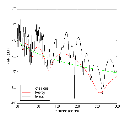
Figure 3.3 represents the path loss attenuation P_r∕P_t = |p₀|² (in dB) as a function of logarithm of distance; it uses h_b = 8 m, h_m = 2 m, f = 2.4 GHz, G_t = G_r = 0dBi, and Γ as given later in §3.3.3. The direct path, using the first term only of (3.7), leads to the simple one-slope free-space model; the complete expression leads to the two-ray model. The figure shows interesting characteristics:

• The presence of a second ray causes great variations: signals can add up or nearly cancel each other, causing deep fades over small distances.
• In close proximity, the overall envelope of power decay varies in 1∕d².
• After a certain cutoff distance (4h_bh_m∕λ) the model approaches power decay in 1∕d⁴.

3.3.3 Reflection and Refraction

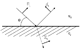
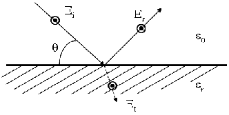
Before moving ahead, we need to take a closer look at reflection coefficients used for indirect rays. The details of this analysis come from boundary conditions for electromagnetic waves traveling between two media. In general these boundary conditions vary with the polarization of the wave and the media permittivities. For a wave impinging on the ground with an angle of incidence θ, the ground reflection coefficient depends on the polarization and is given by equation (3.9):

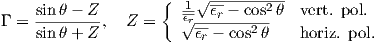(3.9)

Γ is the ground reflection coefficient; Z is the characteristic impedance of the media, as obtained by transmission line theory [76] [19]; θ is the ray angle of incidence (as shown on fig. 3.4); ϵ_r is the complex relative permittivity of the medium: ϵ_r = ϵ_r -j ≈ ϵ_r -j60σλ where ϵ_r is the lossless relative permittivity and σ is the conductivity (in Ω^-1m^-1).

The wave typically has many polarized component to it; even when a transmitter uses vertically polarized antennas, different scatterers in the path may depolarize the wave. Nevertheless, the majority of cellular systems use vertical polarization, which is shown empirically to propagate slightly better in most practical cellular environments. In these cases, the electrical field is near vertical, and the reflection (and refraction) on a surface is shown on figure 3.4.

Similarly, rays bouncing off walls have a reflection coefficient (of course the vertically polarized waves now needs to be considered as impinging the surface with electric field near the surface plane as a horizontally polarized wave does on the ground).

Values for complex permittivities may be used approximately from table 3.1 (from  [19] p. 55, and a few other references); www.fcc.gov/mb/audio/m3/ gives ground conductivity maps for the US.

Further refinements may be thought of regarding the thickness of walls: the ground may easily be considered as an infinite semi-plane, but walls are usually thin enough to make that approximation questionable. ⁶

3.3.4 Multiple Rays

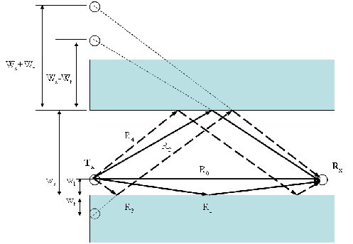
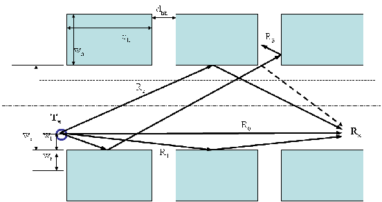
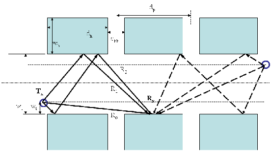
The above 2-ray approach can easily be extended to add more rays  [3]. We may add rays bouncing off each side of a street in an urban corridor, leading to a 6-ray model (with rays R₀,R₁,R₂ each having a direct and a ground bouncing ray). Adding four more rays (bouncing on both sides: R₃,R₄ dashed line in figure 3.6) lead to a 10-ray model.

The direct two rays were computed earlier, the additional rays may easily be obtained from geometry of figure 3.6. Let us assume for instance a street corridor of width w_s, with a transmitter on a light pole w_t from the walls. For simplicity, let us move the receiving point down the street at constant w_t from the wall, in that case distance T_x to R_x represented by R₁ is d₁ = , so, much like equation (3.7), we have:

(3.10)

where l₁ = , and l₁′ = . Γ₁ is the refection coefficient off the nearest wall, and is computed from (3.9), but with angles with respect to the walls.

Additional rays (R₂ and more) can be calculated in expressions resembling (3.10), and added to others in order to produce a multiple-ray model.

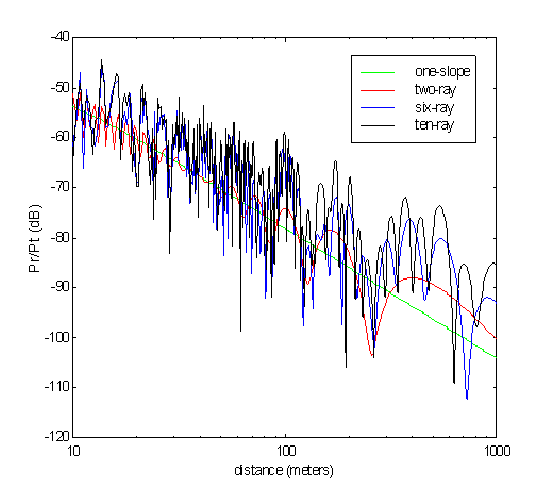
Figure 3.7 shows the increased fading statistic when more rays are taken into account. The figure simply represents the received signal power indicator 20log |∑ _i=0^i=Np_i| as a function of log d₀ for N ∈{0,2,3,5}. For that plot a typical suburban case is taken with street width of 20 feet, and average distance from street to home of w_t = 10 feet (so w_s = 40 feet).

3.3.5 Residential Model

As previously mentioned, that approach is interesting for urban and suburban corridors. We further assume that property lengths and home lengths along the street are approximately identical (say 100 feet and 80 feet respectively). In that case, some rays escape the corridor and never reach the receiver – as illustrated in figure 3.8, R₃ rays escape the urban canyon and never reach the receiver. Taking into account these gaps show a slightly modified model (figure 3.9). Alternatively, instead of examining where rays may escape the corridor, a simplified model may be used that takes into account a power loss proportional to the gaps [42].

3.3.6 Indoor Penetration

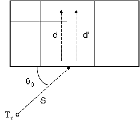
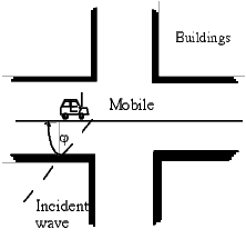
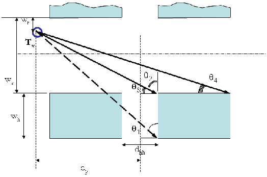
Most cellular towers are placed outdoors, while eighty percent of phone calls are placed indoors. Therefore the problem of how much of the signal strength propagating down the street might be available indoor is of great interest. Grazing angles of incidence are somewhat concerning in urban and suburban corridors. Figure 3.10 shows a typical case where wireless systems (base stations or access points) may be placed on opposite side of the street to provide coverage to residences.

In our previous urban corridor model, the angles of incidences should be restricted to rays illuminating walls (as in figure 3.11). ^{7 8}

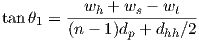(3.11)

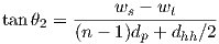(3.12)

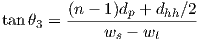(3.13)

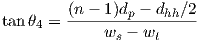(3.14)

Angles of incidences between these values should be used to calculate penetration losses such as:

(3.15)

For instance in a Lakewood neighborhood a light pole is placed every three homes on opposite street sides (i.e. a pole every 6 homes); we get the values in table 3.2 for the furthest home (n = 3, 100-feet properties, 80-feet long homes, 40-feet wide streets, and w_t = 10 feet). And the value L_ge ≈ 10dB is typical for residential areas. (More details in §3.7).

3.4 Classic Empirical Models

Empirical models are simple models that provide a first order estimate for a wide range of locations. A handful of empirical models are widely accepted for cellular communications; these models usually simply consist of computing a path loss exponent n from a set of field data, and deriving a model for path loss (in dB) like:

(3.16)

(where the intercept L₀ is the path loss at an arbitrary reference distance d₀). These models are referred to as empirical one-slope models; their applications and domains of validity are well defined and reviewed later. They generally provide a first estimate used by service provider in wireless systems’ design phase.⁹

A couple of important points should be kept in mind about most propagation models. The first is that large amounts of empirical data are collected usually at cellular or PCS frequencies (800 MHz or 1900 MHz), and extensions to other frequencies are derived as discussed in §3.4.6. The second is that these data points are collected while driving and may not accurately reflect fixed wireless links, which is discussed in more details in §2.10.

3.4.1 COST 231-Hata Model

A one-slope empirical model was derived by Okumura [21] from extensive measurements in urban and suburban areas. It was later put into equations by Hata [22]. This Okumura-Hata model, valid from 150 MHz to 1.5 GHz, was later extended to PCS frequencies, 1.5 GHz to 2 GHz, by the COST project ([23], [24] ch. 4), and is referred to as the COST 231-Hata model; it is still widely used by cellular operators. The model provides good path loss estimates for large urban cells (1 to 20 km), and a wide range of parameters like frequency, base station height (30 to 200 m), and environment (rural, suburban or dense urban).

(3.17)

with the following values:

The parameter a(h_M) is strongly impacted by surrounding buildings, and is sometimes refined according to city sizes:

And an additional parameter C_M is added to take into account city size, and can be summarized for both models as:

Empirical values of the model are limited to distances and tower heights that were used to derive the model; consequently the model is usually restricted to:

• : Base station antenna height: 30 to 200 m
• : Mobile height: 1 to 10 m
• : Cell range: 1 to 20 km

3.4.2 COST 231-Walfish-Ikegami Model

Another popular model is the Walfisch-Ikegami-Bertoni model [30] [31], also revised the COST project ([23], [24] ch. 4), into a COST 231-Walfisch-Ikegami model. It is based on considerations of reflection and scattering above and between buildings in urban environments. It considers both line of sight (LOS) and non line of sight (NLOS) situations. It is designed for 800 MHz to 2 GHz, base station heights of 4 to 50 m, and cell sizes up to 5 km, and is especially convenient for predictions in urban corridors.

The case of line of sight is approximated by a model using free-space approximation up to 20 m and the following beyond:

(3.18)

The model for non line of sight takes into account various scattering and diffraction properties of the surrounding buildings:

(3.19)

where L₀ represents free space loss, L

rtsisacorrectionfactorrepresentingdiffractionandscatterfromrooftoptostreet,andL˙msdrepresentsmultiscreendiffractionduetourbanrowsofbuildings.Thesetermsvarywithstreetwidth,buildingheightandseparation,angleofincidence,andaredetailedintable3.6.

---

Table 3.6: Values for COST 231-Walfish-Ikegami model.

Parameter	Value (dB)
L0	32.4 + 20log(d∕1km) + 20log(f∕1MHz)
Lrts	-16.9 - 10log(w∕1m) + 10log(f∕1MHz) + 20log(ΔhM∕1m) + LOri
w	Average street width
ΔhM	hRoof - hM
LOri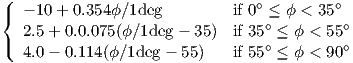
ϕ	Road orientation with respect to direct radio path (see figure(3.12))
Lmsd	Lbsh + ka + kd log(d∕1km) + kf log(f∕1MHz) - 9log(b∕1m)
b	Average building separation
ΔhB	hB - hRoof
Lbsh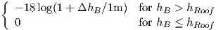
ka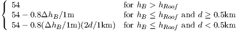
kd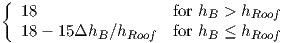
kf

---

The model is usually restricted to:

• : Frequency: 800 to 2000 MHz
• : Base station antenna height: 4 to 50 m
• : Mobile height: 1 to 3 m
• : Cell range: 0.2 to 5 km

3.4.3 Erceg Model

More recently Erceg et al. [32] proposed a model derived from a vast amount of data at 1.9 GHz, which makes it a preferred model for PCS and higher frequencies. The model was in particular adopted in the 802.16 study group [33] and is popular with WiMAX suppliers for 2.5 GHz products, and even 3.5 GHz fixed WiMAX.

(3.20)

where free space approximation is used for d < d₀. Values for L₀, γ, and s are defined in tables 3.7 and 3.8:

The model is usually restricted to:

• : Frequency: 800 to 3700 MHz
• : Base station antenna height: 10 to 80 m
• : Mobile height: around 2 m
• : Cell range: 0.1 to 8 km

The model is particularly interesting as it provides more than a median estimate for path loss: it also gives a measure of its variation about that median value in terms of three zero-mean Gaussian random variables of variance 1 (x,y, and z = N(0,1)).

3.4.4 Multiple Slope Models

Further refinements to these models in which multiple path loss exponents (n₁,n₂) are used at different ranges provide some improvements, especially in heavy multipath indoors environments. For outdoor propagation, two slopes are sometimes used: one near free-space for close points, and another empirically determined. In fact we’ve seen that our 2-ray model could be approximated by a 2-slope model: n₁ = 2 and n₂ = 4 for distances greater than 4h_th_r∕λ.

It seems however that variations from site to site generally are such that these multiple slope improvements are fairly small, and simple one-slope models are generaly a good enough first approximation. More detailed site specific models are required for better results; but they require additional efforts and site specific terrain or building data.

3.4.5 In-building

Indoor propagation often has to be estimated by site-specific models with features specific to a particular building: construction material, wall thickness, floor and ceiling material, all have a strong impact on wave guiding within the building. Some models simply approximate the number of walls and floors, with an average loss for each. See in particular the COST 231 approach in §3.7.

A similar model for indoor environment is the Motley-Keenan model ([2],§7.2), which estimates path loss between transmitter and receiver by a free space component (L₀) and additive loss in terms of wall attenuation factors (F_wall) and floor attenuation factors (F_floor).

(3.21)

Wall attenuation factors vary greatly, typically 10 to 20dB (see table 3.12 in §3.7); and floor attenuation factors are reported to vary between 10 and 40dB depending on buildings. [1]

This model is very site specific, yet sometimes imprecise as it does not take into account proximity of windows external walls, etc; but it can be useful as a guideline to estimate signal strength to different rooms, suites, and floors in buildings.

3.4.6 Frequency Variations

Frequency of operations impacts propagation and path loss estimates. As many models are built on cellular or PCS data measurements, one must be careful about extending them to other frequency ranges.

As seen in equation (3.3) in §3.2, the impact of frequency on free-space propagation is 20logf. Some empirical measurements confirm the trend [37], and the extension is used for instance in the COST-231 Walfish-Ikegami model.

Empirical evidence also shows however that frequency extensions are obtained by adding a frequency dependence in f^2.6 (or a 26log f term in dB) as suggested by [40], and used for instance in the Okumura-Hata model [22] and the 802.16 contribution [33].

Finally other important aspects have a significant impact as frequency changes. Spatial diversity gain typically improves with frequency since spatial separation increases when related to wavelength ([41] shows a 2dB diversity gain from cellular 850 MHz to PCS 1.9 GHz). Doppler spread and impact on symbol duration should also be studied separately and may have a significant impact on a change of frequency [43]. Impact on in-building penetration is examined further in §3.7.

3.4.7 Foliage

Foliage attenuates radio waves and may cause additional variations in high wind conditions [44]. Propagation losses and path loss exponents vary strongly with the position of transmitter with respect to the tree canopy; they also vary with the types and density of foliage, and with seasons. [45][46][47][48][49]

We will report in a later chapter on the impact of foliage for fixed wireless links at 3.5 GHz, in a suburban area as foliage grows from the winter months into the spring (see figure 10.9). Studies have been published at different frequencies; some identify empirical attenuation statistic with Raleigh, Ricean, or Gaussian variables, others derive excess path loss, or attenuation per meter of vegetation.

As a rule of thumb, at frequencies around 1 ot 6 GHz single tree causes approximately 10-12 dB attenuation, and typical estimates are 1-2 dB/m attenuation. Deciduous trees in winter cause less attenuation: 0.7-0.9 dB/m. (See table 3.9.)

Another common models for vegetation proposes an empirical exponent both for distance and frequency; thus approximating vegetation loss by L(dB) = Af^αd^β, where A,α, and β parameters vary with the type and density of vegetation. See figure 3.13 taken from [50].

3.5 Further Modeling Work

The above models are in a sense simplistic as they focus on path loss as a function of distance. Although these models work well in large cellular coverage prediction, they are often deemed insufficient for smaller cells such as wireless LAN’s, especially where multipath is dominant, as in a heavy urban environment or indoor environment.

An interesting and important activity around propagation modeling is the COST project (COperation europénne dans le domaine de la recherche Scientifique et Technique), a European Union Forum for cooperative scientific research that has been useful in focusing efforts and publishing valuable summary reports for wireless communications needs.

COST 207

“Digital Land Mobile Radio Communications”, March 1984 - September 1988, developed channel model used for GSM,

COST 231

“Evolution of Land Mobile Radio (Including Personal) Communications”, April 1989 - April 1996, contributed to the deployment of GSM1800, DECT, HIPERLAN 1 and UMTS, and defined propagation models for IMT-2000 frequency bands [24]

COST 259

“Wireless Flexible Personalised Communications”, December 1996 - April 2000, contributed to wireless LAN modeling, and 3GPP channel model [25]

COST 273

“Towards Mobile Broadband Multimedia Communications”, May 2001 - June 2005, which contributed to standardisation efforts in 3GPP, UMTS networks, provided channel models for MIMO systems [26]. That work was later continued in the COST2100 group[27] in particular to provide further MIMO advances for the wireless industry.

Finally, new interesting activities of research and modeling are taking place at higher frequencies, in millimeter-wave for mobile use with 5G [28][29].

3.6 Dispersive Models

Modern radio systems now make extensive use of multiple paths between transmitter and receiver, even deploying multiple antenna systems (such as MIMO). These systems require more than path loss estimates, as path loss is sensibly the same between transmitting and receiving antenna systems. MIMO channel models are therefore much more complex; several approaches have been used, such as different groups of delayed paths. Of particular interest are the 802.16 model [33], the 802.11n and ac models [34] for various indoor models (from the 802.11n task group on channel modeling), or [38] for mobile cellular models.

IEEE 802.16e and SUI

The work of 802.16 and Wimax provided the first widespread models with interesting multipath considerations and convenient matlab simulations [33]. The work starts with six typical environments modeled by six Stanford University Interim (SUI) channel models. These models are described in terms of terrain types (and propagation from §3.4.3), amount of Doppler, delay spread, and fading statistics.

One way of modeling transmission delay (beyond a simple delay spread value) is to consider a series of successive impluses, each delayed and attenuated. This is referred to as the tapped delay line model. The SUI models define 6 different types of environments, with different tap delays, Doppler effect, and fading statistics: in that manner the model represent different scenarios: pedestrian/vehicular, urban/suburban/rural, indoor/outdoor, etc.

IEEE 802.11n

The IEEE task group TGn produced a series of models [34] for 802.11n (and ac) for LAN applications at 2.4GHz and 5GHz. Consequently these models focus on pedestrian mobility; the group presents six different models (named A to F) aim at describing typical LAN environments, with generally much more multipath than many outdoor cellular environments.

---

Table 3.10: TGn channel models A to F are used to model MIMO systems in different environment, with different RMS delay spreads (σ_τ in nanoseconds – see table 4.2 in §??).

Model	στ(ns)	Environment	Example
A	0	Direct	Cabled
B	15	Residential	In room or room-to-room
C	30	Res. or small office	Conference rooms, classrooms
D	50	Typical office	Cubicles in open office space
E	100	Large office	Large office space, multi-floor
F	150	Large space	Indoor large hangars, outdoor campus / urban

---

---

Table 3.11: TGn channel models A to F use two slopes n₁ = 2 near transmitter, and different values of n₂ beyond a critical distance d₀. They also estimate different log-normal shadowing standard deviations σ₁ = 3dB near transmitter, and higher values σ₂ beyond d₀.

Model	d0(m)	n1	n2	σ1	σ2
A	5	2	3.5	3	4
B	5	2	3.5	3	4
C	5	2	3.5	3	5
D	10	2	3.5	3	5
E	20	2	3.5	3	6
F	30	2	3.5	3	6

---

3GPP SCM

The 3GPP spatial channel models (SCM) [38] focus on 3G and 4G applications such as UMTS and LTE, in 5MHz channels around 2GHz. There are again different models, based on environment, speed etc, typically modeling N delayed multipaths, each comprised of M subpaths (in typical urban and suburban environments, the model uses N = 6,M = 20). Different parameters are also given for different environments (suburban macrocell, urban macrocell, and urban microcell): pathloss (LOS and NLOS), antenna beamwidth, delay statistics, log-normal shadowing, angles of arrival distribution, etc.

Important work on correlation between these multiple path is also presented, as it is crucial to estimating the MIMO rank important for system capacity (see §9.1.3). The 3GPP spatial channel models (SCM) report [38] is a wonderful source of many other parameters and typical values very useful for any propagation aspects of propagation for mobile communication systems.

3.7 In-Building Penetration

Sending RF signal into buildings means additional building penetration loss in the link budget. Indoor penetration measurements are difficult to perform, and difficult to compare from one experiment to another. Difficulties arises mostly from the fact that indoor and outdoor environments are so different that the method of data collection may cause large variations between the two environments; the following parameters have an influence: antenna beamwidth, angle of incidence, outside multipath, indoor multipath, distance from the walls, etc.

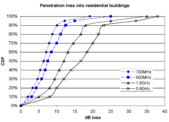
Measurement campaigns show that the distribution of building penetration loss is close to log-normal [17], a Gaussian function is a good approximation of the cumulative distribution function (CDF) of indoor measurements. The mean μ_i and standard deviation σ_i of indoor penetration loss vary with frequency, types of homes, and environment around the homes. Variations also depend on the location within the building (near an outside wall, a window, or further inside). Finally the angle of incidence with the outside wall also has a significant impact.

With that in mind, we can consider that wireless systems with in-building penetration have a shadowing statistic with a log-normal random variate which combines two independent log-normal variates: the outdoor shadowing (detailed further in §4.1 with standard deviation σ_o) and the in-building loss (with standard deviation σ_i). ¹⁰ And the aggregate random variate is also log-normal distributed, and has a standard deviation σ = .

3.7.1 In-Building Models

The COST project proposes models for indoor penetration ([24] §4.6) with variations of angle of incidence. The COST 231 indoor model simply uses a line-of-sight path loss with an indoor component:

(3.22)

where S is the outdoor path, d is the indoor path, and

(3.23)

where L_e is the normal incidence first wall penetration; the next term represents the added loss due to angle of incidence θ and is sometimes measured over an average of empirical values of incidence, in which case it may be noted L′_ge = L_ge(1 - sinθ)²; and the last term max(Γ₁,Γ₂) aims at estimating loss within the building, whether going through walls or in a corridor.

Since angles of incidence are not always known the estimate L′_ge = L_ge(1-sinθ)² is sometimes more convenient. As a rough estimate for angles of incidence between -π∕2 and π∕2 lead to the following:

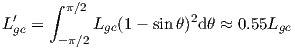(3.24)

Empirical values of L′_ge are reported to be ≈ 5.7 - 6.4 [54] for residential areas, therefore we may use L_ge ≈ 10dB. For urban environments, COST-231 reports L_ge ≈ 20dB.

As for further interior loss, the COST model distinguishes between propagation through walls and propagation down coridors. Through n_i interior walls of loss L_i each: Γ₁ = n_iL_i. In a corridor: Γ₂ = α(d′- 2)(1 - sinθ)², with an empirical propagation loss α = 0.6dB/m.

Typical values for the model reported in [24] and [54] are summarized in table 3.12.

3.7.2 Residential Homes

In most residential and suburban environments, surfaces involved are mostly made of glass, bricks, wood, and drywall. Penetration is often dominated by paths through windows and roofs, loss are relatively low and go up with frequency.

Precise characterization of in-building penetration is difficult, a rough approximation of an average penetration loss μ_i around 10 to 15 dB and a standard deviation σ_i around 6 dB seems to be the norm in published studies. Table 3.13 and figure 3.7.2 summarize some published results for residential homes.

3.7.3 Urban Environments

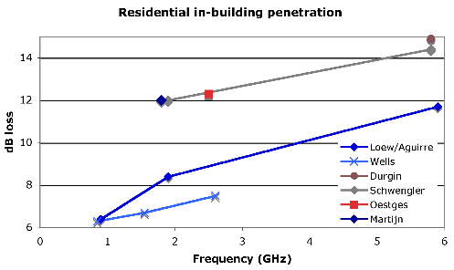
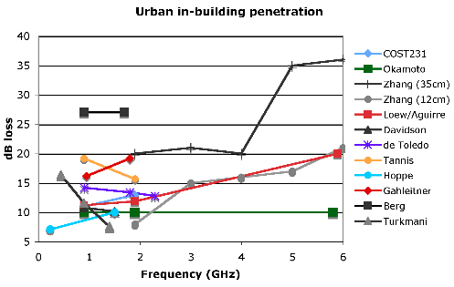
In dense urban areas experiments show different trends as illustrated in figure 3.7.2: some papers show penetration loss increasing with frequency [51][55]; some claim loss are independent of frequency [64][57]; others show a decrease with frequency [61][60][59].

Furthermore the variations between buildings and types of environments nearly always exceed the frequency variations. These environments are dominated by reflections off metal reinforced concrete and heavily reflective glass. In case of high-rises, penetration also depends on the floor and height of neighboring buildings or clutter.

3.7.4 In-Vehicle Loss

Given the mobile nature of wireless communications, penetration loss into vehicle is important as well. Precise characterization of in-vehicle penetration is difficult as well, and varies with type of vehicles, frequency, polarization, antenna placement in the vehicle, and direction of incidence. [66][67][68] An average penetration loss μ_v around 8 dB and a standard deviation σ_v around 3 dB seems to be the norm in published studies – see table 3.14.

Just like in-building penetration, in-vehicle penetration is a log-normally distributed random variate (with standard deviation σ_v), it is independent of the outdoor large scale shadowing statistic (σ_o), ¹¹ and the aggregate loss is log-normal distributed with standard deviation σ = .

3.8 Homework

1. At the beginning of section 3.2, we start to derive a free-space model from Friis’ equation. (a) Rederive in details the Friis’ formula (3.2). (b) Assume in the above that G_t = G_r = 1 (=0 dBi), derive (3.3).
2. Find the paper [32] by V. Erceg & al. “An Empirically Based Path Loss Model for Wireless Channels in Suburban Environments”, in IEEE Journal on Selected Areas in Communications, Vol. 17, No 7, July 1999. This popular paper for PCS propagation modelling and design deserves some attention. Read it and answer the following questions:
   1. Summarize data collection campaign methods and size.
   2. Summarize key findings.
   3. A key finding is that path loss exponent variations are Gaussian, how is that proven in the paper?
3. Plot path loss prediction versus distance and log distance for a cellular system you are designing with the following assumptions: PCS frequency (1900 MHz), base height 20 m, mobile 2 m, suburban area, flat terrain with moderate tree density.
   1. Use and compare the 3 following models: Free space, COST 231-Hata, & Erceg (use a median path loss: i.e. x=y=z=0)
   2. Using typical 140 dB maximum allowable path loss for a CDMA voice system, what is the range (cell radius) according to these models?
4. Repeat the above problem with unlicensed frequency 5.8 GHz and a link budget of 120 dB. Compare. (Use the same models, including COST 231-Hata and Erceg models even though the frequency exceeds their domain of validity.)
5. Compare the received power level of free-space (n=2), and 2-ray models for a PCS signal (1900 MHz; use h_b = 8 m, h_m = 2 m). Write a program (in any language of your choice) to plot a graph of power level versus log of distance (from 10m to 10km). Submit code with comments and explanations, and a resulting figure.
   1. First assume a simple perfect reflection Γ = -1
   2. Then use the actual Γ given for a vertical polarized wave. Is the difference significant?
   3. What cell site radius would be ideal for a system design? Why?
6. Plot and compare on a same graph the propagation estimate for a radio system at 2.4 GHz and another at 5.8 GHz (all other parameters being equal); use h_b = 8 m, h_m = 2 m; use a) the two-ray model from §3.3.2, b) the 6-ray model from §3.3.4. Point out the main differences.
7. Find and read the three papers referenced for in-vehicle penetration [66][67][68], as well as any other such reports or paper if you can.
   1. Produce a table like 3.14 with clear references, but with more details.
   2. Define average values (for mean and standard deviation) that you would recommend using for 700MHz, 800MHz, 1.9GHz, 2.4GHz propagation into vehicles. Justify.
8. Find and read reference [33].
   1. Implement the software emulations from appendix B (e.g. using Matlab) and produce a simulation of the fading for SUI-3 with omnidirectional antenna at in figure 1 of that appendix B.
   2. Play with some parameters of the simulation, and submit one more, and analyze some noticeable differences.
9. This problem studies the main differences in link budget to be expected between cellular and PCS systems. This problem is inspired from a 1999 paper by Chu and Greenstein [40] — feel free to refer to it for further details, but some analyses have been simplified, and some values were changed, so do not use any numerical values from the paper or this problem.

   Cellular and PCS systems are usually FDD, thus operating at different frequencies for uplink and downlink. Still in this problem, we neglect that small difference, and we assume cellular frequency to be 800MHz, and PCS frequency to be 1900MHz.

   1. Typical path loss models like one slope models do take into account the variation due to frequency. For simplicity we use here the frequency variation seen in the free space model. Evaluate that variation (in dB).
   2. Calculate the link budget difference between cellular and PCS. Give your answer as LB(cellular)-LB(PCS) in dB.

      We’ll try in the following questions to make up for that difference.

   3. Antenna gain can make up some of that difference. Let’s assume that we use antennas of the same size, meaning that they have the same effective area A_e = G_aλ²∕(4π). What antenna gain difference ΔG_a is there between cellular and PCS?
   4. Another improvement is that of diversity. We consider receive diversity at the base station only; handset receive diversity will be considered negligible. Diversity gain depends (inversely) on the correlation ρ between the signals:

      (3.25)

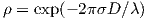      (3.26)

      where λ is the wavelength, D is the antenna separation, and σ is the standard deviation of the angle of arrival, which is difficult to estimate, and we’ll use an empirical estimate of 1 degree, which means σ = 0.0175 rad in the formula above.

      Calculate ρ at both frequencies for 6-feet antenna separation. Calculate ΔG_d, the diversity gain difference between cellular and PCS.

   5. Another difference may be the impact of vegetation in the cell: a simple vegetation attenuation formula is sometimes: L_v(dB∕km) = 1.33f^0.284 with f in MHz. We’ll consider that a cell is on average 1km radius, therefore we’ll use L_v for our link budget. Calculate the difference in vegetation loss between cellular and PCS.
   6. Noise at the receiver is another important consideration. Handset noise is considered identical, but base station noise parameters vary. The main difference seems to be that ambient noises (mostly man-made) is higher at 800MHz, that impact on the receiver can be approximated (in dB) by P_mm = 2.4 - 2.3log(f∕100) with f in MHz. Calculate that difference between cellular and PCS.
   7. In-building penetration is also likely to vary: from the relevant figure in the class notes, estimate the difference in building penetration loss for the 90th percentile of the CDF. (Meaning the additional loss we should consider to account for 90% of residential buildings.)
   8. Summarize and calculate the link budget difference seen in all questions above. That is the link budget difference between cellular and PCS for the uplink (reverse link).
   9. Conclude and comment about the value of cellular vs. PCS spectrum — e.g. quantify coverage.
10. Repeat the previous problem to compare 700MHz and AWS (1700MHz) spectrum.

Copyright ©2019 Thomas Schwengler. A significantly updated and completed 2019 Edition is available.