Copyright ©2019 Thomas Schwengler. A significantly updated and completed 2019 Edition is available.

Chapter 10
Wireless System Performance

10.1 Wi-Fi System Performance

Wi-Fi systems and services are evolving from simple stand-alone access points (AP) to complex networks. We review here Wi-Fi data rates, and examine some extensions to larger systems.

10.1.1 Data Rates

Wi-Fi systems rely on IEEE 802.11 a, b, g, n, and ac. Early systems use frequency hopping schemes and direct spread spectrum, but most systems now focus on the OFDM physical layer. Their data rate of is determined by the type of modulation and coding: from BPSK 1/2 to QAM256 5/6. Physical data rates for 802.11a/g are quoted up to 54 Mbps, but maximum payload or user data throughput cannot exceed 36 Mbps, and actual measured throughput vary with suppliers (up to 30 Mbps); and interoperability between suppliers introduce even greater variations.

Table 10.1 summarizes typical data rates observed in a 20 MHz TDD 802.11g channel. These results were measured with low interferences and all client devices near the AP and within the same room, leading to system operations at maximum modulation.

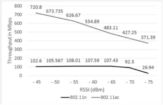
802.11n and ac further increase throughput by various new schemes such as: lower guard interval, higher coding rate, greater channel width, and MIMO. Here again actual throughput are lower (of the order of half the PHY rate).

10.1.2 Municipal Wi-Fi

Municipalities have tried a few years back to deploy affordable wireless networks free to use for their citizens. The common opinion is that Wi-Fi networks would be cheaper than other mobile wireless products because: 1) spectrum is free and 2) Wi-Fi client devices are free since they are part of laptops and tablets. Other arguments include 3) access points are cheap (when compared to cellular equipment) and 4) they are easier and cheaper to install (when compared to cellular towers)

The first two facts are a great advantage for Wi-Fi since they are an important part of the cost of providing service, but come at the cost of a fairly weak link budget, which greatly impacts operations. [154]

There are other key cost factors of wireless networks, including: cost of acquisition of new customers, including activation, billing, and the distribution of client device. Other considerations include usage needs and patterns, especially around indoor coverage. The majority of data need is still indoor (at home or at work). Indoor coverage from outdoors access points are very difficult to build reliably (recall link budgets and indoor penetration).

Outdoor needs have been well met by mobile devices, but recent demand for capacity is pushing again for small cells (including Wi-Fi). Fixed outdoor usage is of course limited by weather and temperature, which limit revenue opportunities.

10.1.3 Radio Parameters Analysis and Modeling

Wi-Fi coverage and capacity considerations are similar to those of any cellular network, and even more stringent since only 3 non-overlapping channels are available for a reuse factor of 3 (Although reuse factors of 4 with channels 1, 4, 8, 11 have been rolled-out, e.g. in Longmont).

In an initial design phase, a simple one-slope model and low-resolution terrain data suffice for a rough estimate to qualify customers. As operations progress, actual measurements are compared to predictions and the process is refined further.

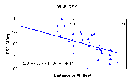
The variations in RSSI as a function of distance were measured in a residential neighborhood and are shown here. Note that measurements taken in the street may show a fairly low slope (due to the street corridor effect).

10.1.4 Throughput Measurements

Throughput is affected by distance, shadowing, and interferences. In most cellular trials, mobile data is collected, which makes it impossible to quantify variations over long periods of time for a given location. In a population of fixed location, however, a measured standard deviation over a long period may be useful in predicting seasonal changes in the radio channel.

10.2 WiMAX System Performance

The WiMax standard appeared in 2006 as a cost-effective solution for fixed wireless access.

10.2.1 Data Rates

IEEE 802.16 and WiMAX profiles allow for several radio channel bandwidths, which lead to very different data rates. WiMAX systems have modulation and coding ranging from BPSK 1/2 to QAM64 3/4. Measured throughput vary with suppliers: a degradation of 40% to 50% is often observed compared to theoretical throughput. Table below summarizes typical data rates observed in a 3.5 MHz FDD channel (also see figure 10.9 on page §). Actual data results vary with suppliers, and interoperability between suppliers introduce even greater variations.

Of course different profiles and channel widths lead to different throughput results. An unlicensed TDD 10 MHz channel profile for instance has the advantage of adapting to asymmetrical data demand. Similar benchmark tests show that such a system is also capable of throughput around 8 Mbps (see §10.2.5 and specifically figure 10.10). Interferences from other cells (co-channel interferences) strongly impact actual rates, especially at cell edge [156] [157].

To estimate system performance, Stanford University Interim (SUI) models are used to create models that emulate different terrain types, Doppler shift, and delay spread as summarized in table. Terrain Types are (from [32]) defined as follows. A: the maximum path loss category, hilly terrain with moderate-to-heavy tree densities; B: the intermediate path loss category, hilly with light tree density or flat with moderate-to-heavy tree density; C: the minimum path loss category, mostly flat terrain with light tree densities. These terrain categories are also used to model obstructed urban, low-density suburban, and rural environments respectively.

10.2.2 Experimental Data

Fade emulators in lab environment can recreate the above SUI fading profiles to evaluate radio systems performance in different fading environments.

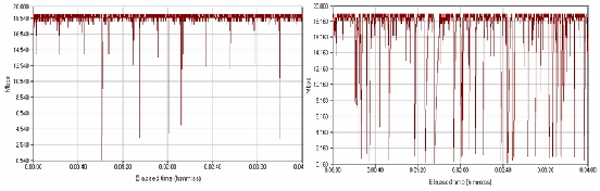
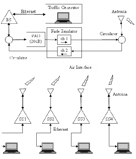
Radio system under test comprises one base station (BS) and several subscriber stations (SS’s). Different fading channels are programmed in the channel emulator. The Fading emulator emulates two separate channels (forward and reverse links), each comprised of several multipaths, each of which is independently faded and delayed. Fade statistics for the direct path are either Rayleigh or Ricean, delayed paths are attenuated and Rayleigh faded as specified by SUI models. In this test, the unidirectional nature of the fade emulator forces us to separate transmit and receive paths (with circulators). Additional attenuation (pad) is added where necessary. Finally a traffic generator is wired to the BS and laptops are wired to SSs for data collection. Figure 10.6 shows the detailed setup.

10.2.3 Radio Parameters Analysis and Modeling

In an initial design phase, a simple one-slope model and low-resolution terrain data suffice for a rough estimate to qualify customers. As operations progress, actual measurements should be compared to predictions and the process should be refined further.

A path loss estimate is derived from RSSI measurement (and transmitted power level, which depends on base station power, cable loss, antenna pattern, and even on the deviation from boresight of the sector’s antenna. Path loss estimates are represented in figure 10.7.

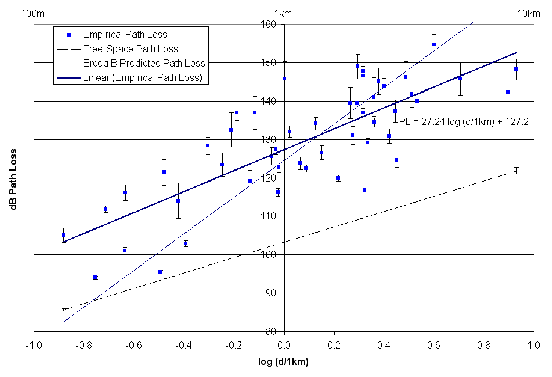
Approximation of path loss to a one-slope model leads to the following equation:

(10.1)

with d₀ = 1 km. The trial environment is compared to typical cellular models as discussed below.

• Path loss exponent is approximately n = 2.7. The Walfish-Ikegami model for line of sigh in urban corridors predicts n = 2.6. Other reports have shown similar results for 3.5 GHz: [71] reports values of n between 2.13 and 2.7 for rural and suburban environments, [73] reports n = 3.2. But many other models predict higher exponents n between 3.5 and 4.5. (See path loss exponents in table 1.1).
• Otherwise, approximations are fairly good with Erceg-B and C models. Erceg-B is the best fit and is represented on figure 10.7.

A classic approach to compute slope estimate is a least square error estimate, in which a set of error terms {e_i} is defined between each data point and a linear estimate. Minimizing the sum of these errors yields the slope and intercept, which intuitively gives a good approximation of the data set. That method also benefits from the following important properties [158]:

1. Least square estimated slope and intercept are unbiased estimators.
2. Standard deviations of the slope and intercept depend only on the known data points and the standard deviation of the error set {e_i}.
3. Estimated slope and intercept are linear combinations of errors {e_i}.

From the last point, an assumption that the errors are independent normal random variables (as in a log-normal shadowing situation) leads to a slope and intercept also normally distributed. If we assume more generally that the data points are independent, the central limit theorem means that the estimated slope and intercept tend to be normally distributed. For the last assumption to be true, very low correlation of the wireless channel must exist between data points. This is the case when data points are measured at fixed locations tens or hundreds of meters apart, or, in a mobile cellular environment, from one cell to another.

The important point is that path loss exponent is approximated by a normal (or Gaussian) random variable. We also verify a few more key findings as in [32], for a 3.5 GHz fixed link:

1. Free-space model (PL₀ = 20×log) works well within 100 m.
2. Path loss exponent depends strongly on height of transmitter (mobile height being more or less constant throughout).
3. Variations around median path loss are Gaussian within a cell (Log-normal shadowing), with standard deviation σ ≈ 11.7 dB.
4. Unfortunately, our limited number of cells does not allow us to quantify the nature of the variations of σ over the population of macro cells.

10.2.4 Throughput Measurements

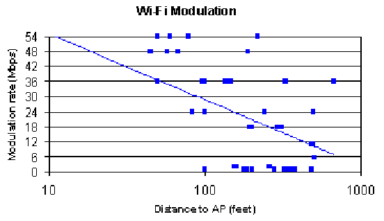
Throughput is affected by distance, shadowing, and interferences. RSSI and SNR have a direct impact on the modulation and therefore on the throughput of the wireless link. That throughput is graphed as a function of distance in figure 10.8.

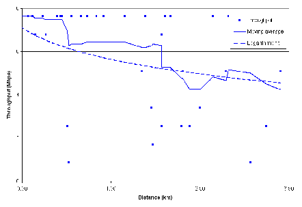
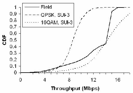
In fact, modulation and throughput change from time to time, their statistical distribution is illustrated in figure 10.9 (and 10.10). When compared to controlled fading environments described in 10.2.1, fading statistics in suburban areas show close correlation with SUI models 3 and 5, and throughput density functions near those of 16QAM 3/4 in such fading environments [159].

Finally we examine the standard deviation of measured signal strength over long periods of time for a given location: typical standard deviations in fixed links over several months vary between 1 and 6 dB, more as leaves come out if deciduous trees are present in the path. Trial data also show that the standard deviation tends to increase with distance, on average:

(10.2)

with d₀ = 1 km.

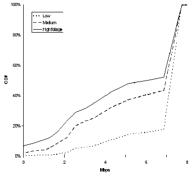
Seasonal variations are moslty noticeable as leaves come out. The impact on the link budget has been reported for fixed wireless links [47] and in different wind conditions [44]. We measure some variations of the path loss exponent, the intercept, and the log-normal shadowing. In many cases the wireless system can adapt to these variations, but in some marginal locations where link budget nears the maximum allowable path loss, throughput is affected. As shown on figure 10.9, low bit rates are affected the most by changes in foliage.

10.2.5 Unlicensed WiMAX

Unlicensed WiMAX operates at 5.8 GHz, in 5 or 10 MHz TDD channels (using 256 or 512 FFT respectively). Their performance is illustrated in this section. Comparison between field and lab data shows that measurements made downtown Denver match a SUI-3 model, and that adaptive modulation seems to maintain a radio link between QPSK and 16QAM.

Copyright ©2019 Thomas Schwengler. A significantly updated and completed 2019 Edition is available.