
Copyright ©2019 Thomas Schwengler. A significantly updated and completed 2019 Edition is available.
In the 1960’s microwave links started to be used for communications on a large scale, and significantly impacted the telecom industry. Newcomers like Microwave Communications, Inc. (MCI) impacted both technical and regulatory aspects of the telecom industry. During the following decades microwave links have been used throughout the United States and globally to build long-distance networks where wired lines were too costly or too time consuming to build. In the last few years, microwave and millimeter-wave radios have come down dramatically in size, and cost; they have also increased in capacity. As a result, fixed microwave radio links are an excellent solution for many new broadband applications, such as Ethernet transport, including to cell sites.
Cell sites provide increasing data rates and therefore need increasing backhaul capacity. A few Megabits per second were sufficient for 2G, and could easily be provided to any cell site by ordering T1 (or DS1) circuits from a local carrier.1 Subsequent generations, however, regularly increase data demand and backhaul requirements, which becomes increasingly expensive and sometimes impractical to provide by increasing DS1 circuits. In these instances microwave radio links can be very useful.
To achieve high data rates, backhaul techniques use microwaves and millimeter-waves at frequencies above several gigahertz (GHz), or even infrared lasers in the terahertz (THz) range. As a result, backhaul links are often limited to line-of-sight propagation, and may suffer from atmospheric impediments.
We have seen in section 1.3.2 that several bands of spectrum are available in the US for unlicensed (or license exempt) communication. These bands are also used for point to point applications such as backhaul. As seen above, they are governed by FCC Code of Federal Regulations Title 47 (CFR 47) part 15 rules. Device power and EIRP are limited in order to alleviate interference issues, equipment must be approved by the FCC (mainly to verify power levels and emission masks).
The ISM bands and UNII bands (at 900MHz, 2.4GHz, and 5GHz), popular for indoor devices and wireless LAN, are also widely used for longer range fixed broadband links. In addition, a few more fixed wireless unlicensed bands exist in higher spectrum; these bands benefit from heavy atmospheric absorption, which limits range of operations but also unwanted interferences.
In addition, infrared links can be used for communications. At higher frequencies, radio spectrum approached the range of visible; its advantages are that several THz of spectrum are available for applications exceeding Gbps. In that range, operations are usually referred to as free-space optics; and bands are measured in wavelength rather than frequency. Different scattering and atmospheric considerations are involved: dust and fog become dominant considerations rather than water vapor content and rain.
In the US, the Code of Federal Regulations Title 47 (CFR 47) part 101 regulate Fixed Microwave Services. Part 101 makes several bands of spectrum available for use for fixed microwave service. Several bands of spectrum are available in several channel width (10 to 80MHz) and cover a fairly large portion of spectrum in order to allow carriers to design links for a wide choice of capacity and distances. Traditionally, the industry has used bands of spectrum at 6GHz, 11GHz, 18GHz for long-haul links. More recently bands at 23GHz and 24GHz were made available: although they suffer from higher atmospheric attenuation, they can be useful for multiple reasons: lower bands may be congested in that area, smaller antenna dishes (at higher frequency) may be more convenient, and finally their channel bandwidth is wider and allows for higher capacity than lower bands. The FCC also allocated millimeter-waves frequencies for higher capacity point-to-point licenses, albeit at shorter distances: 71-76GHz and 81-86GHz bands are now available for fixed service. And 92-95 GHz is also available (except for 94-94.1GHz reserved for military applications).
Under part 101 rules, licenses are available for registration from the FCC and may operate equipment approved for CFR 47 part 101 use. Typically, a carrier wanting to use one of these licenses has to register the location of the link, and for a nominal fee can lease a block of spectrum. Licenses follow a few simple rules:
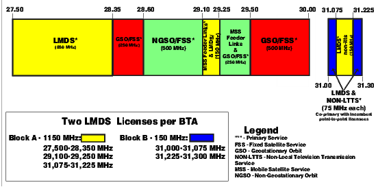
The FCC also made available a number of other licenses for fixed wireless service; some licenses were given to industry pioneers at 24GHz and 39GHz, and in 1998 spectrum was auctioned for Local Multipoint Distribution System (LMDS). LMDS spectrum offers 1300MHz of spectrum (between 28GHz and 31GHz, allowing up to 30dBW/MHz EIRP), which can be used for point-to-point links much like part 101 spectrum, but also for point-to-multipoint systems. The ability to roll-out point-to-multipoint systems, in which one hub may cover an entire area, was seen as a new and efficient way to provide fixed microwave service in many populated areas.
Telecommunications companies combined these licenses to extend their fiber networks. The life of point-to-multipoint systems was very short, however, and most long links today are point to point. Nevertheless the amount of spectrum available, and the time to market advantage make LMDS licenses a useful asset, and may see renewed interest for short high-throughput applications – see §5.6.
Recently, a new part 30 was created for Upper Microwave Flexible Use Service (UMFUS), which relates to fixed and mobile use of frequencies above 24GHz for expected 5G use [14].
LMDS and 39 GHz were regulated in part 101, and with new mobile flexibility are moving under this new part 30. Power is limited to 75dBm per 100MHz EIRP at the base station (average power of the sum of all antenna elements), 43dBm EIRP for mobile, and 55dBm for fixed transportable stations (e.g. in homes and cars). Duplexing rules have also been changed to be very flexible.
Microwave radio links operate above 6GHz, and are therefore highly affected by obstruction, so much so that long range microwave links nearly always require line of sight. Consequently a free-space model is a good way to start microwave propagation modeling. That will however not be enough: given the higher frequencies and longer distances involved, we’ll also have to take into considerations the impact of obstructions, atmospheric variations, and weather (especially rain).
Recall from section 3.2 and equation (3.3) that free space path loss at a distance d can be expressed as:
 | (5.1) |
where f0 = 1 MHz, and d0 = 1 km. These reference values are arbitrary and chosen to be convenient to use values in MHz and km in the formula. (And recall that the constant 32.45 changes if the reference frequency f0 and the reference distance d0 are chosen to be different.)
Diffraction loss is a very important consideration in the design of microwave links. It depends on the path clearance, which depends on the type of terrain, the amount of obstructions, and vegetation. For a given path clearance, the diffraction loss will vary from a minimum value for a single knife-edge obstruction to a maximum for smooth spherical obstructions. Practical obstructions do not resemble knife edges, but convenient approximation formulas exist for them, and are often simply used to estimate obstruction loss.
Most of the energy on a microwave link is concentrated within the first Fresnel region, and diffraction loss are often calculated as a function of obstruction with respect to the first Fresnel zone. Fresnel zones are zones delimited by prolate ellipsoids of revolution with transmitter and receiver as the two foci; the nth Fresnel zone is the loci of points with an excess path between (n- 1)λ∕2 and nλ∕2 over the direct path. Odd Fresnel zones (especially the first) carry important propagation energy, and are therefore essential in the calculation of obstruction loss.
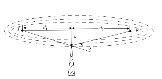
Let’s call h the height difference (in m) between the path trajectory and the most significant path blockage; so h is positive if the top of the obstruction is above the virtual line-of-sight, and negative if the obstruction is below as is the case in figure 5.2. 2 Fn, the radius of the nth Fresnel ellipsoid can be approximated by the following formula:
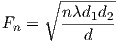 | (5.2) |
with λ: wavelength, d = d1 + d2: total path length, and d1,d2: distances from radio transceivers to the obstruction. It is convenient to summarize the first Fresnel zone radius in meters (m) to:
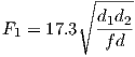 | (5.3) |
with f: frequency (in GHz), d: path length (in km), and d1,d2: distances (in km) from radio transceivers to the obstruction. (For the latter equation, be aware of the various units: m, km, GHz)
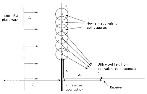
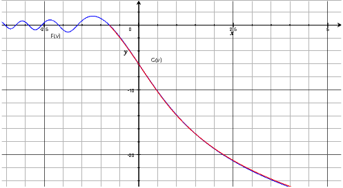
A common approach is to consider a perfectly conducting knife edge obstacle blocking the propagation path. We then consider Huygens equivalent point sources above the obstruction, each contributing to the field at the receiver (see figure 5.3). We define a parameter ν:
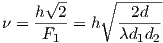 | (5.4) |
The resulting field is shown to be Er∕Et = F(ν) with :
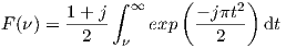 | (5.5) |
The expression can be calculated in terms of Fresnel cosine integral
C(x) = ∫
0xcos dt and sine integral S(x) = ∫
0xsin
dt and sine integral S(x) = ∫
0xsin dt:
dt:
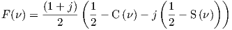 | (5.6) |
and the diffraction gain (in dB) is defined as
 | (5.7) |
which is now fairly easy to compute with modern tools since many mathematical software packages include functions such as Fresnel integrals.
When simpler approximations are required, the diffraction gain is simply taken to be 0dB for small obstructions (h∕F1 ≤-0.55, or ν ≤-0.77). For larger obstructions, a convenient approximation of the diffraction gain (in dB) is given by [92]:
 | (5.8) |
Figure 5.4 shows how close the estimates compare; the two curves are nearly indistinguishable.
It should be noted however that empirical measurements of diffraction obstacles are worse than those modeled by knife edge (mountains or buildings for instance are often not similar to a knife edge, and empirical estimates for diffraction loss are sometimes taken to be (in dB) Ad = 10 + 20h∕F1. Note the 10dB loss when the obstruction reaches the line of sight instead of 6dB for the knife edge model – also see Figure 5.5.
Generally, practical microwave designs tend to clear the first Fresnel zone. In some cases, however, engineers refer to clearing 55% of the first Fresnel zone; which really means that 55% of the radius of F1 below the radio path is not obstructed (h∕F1 = -0.55), which corresponds to a 0dB diffraction loss.
The earth atmosphere is a complex gaseous mixture and has various effects on radio propagation such as attenuation and depolarization.
Generally air pressure decreases with elevation thus decreasing refraction index or relative electric permittivity of air.
The index of refraction of air is very close to 1 (index of refraction of vacuum), so in order to avoid using a number so close to 1, the radio refractive index (or radio refractivity) is defined as [94]:
 | (5.9) |
for which an empirical formula is:
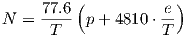 | (5.10) |
where T is the temperature in Kelvin, p is the atmospheric pressure in hPa (or mbar), and e is the the water vapor pressure, also in hPa. An empirical formula can be expressed as a function of height by the exponential law:
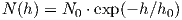 | (5.11) |
where N0 is the average value of atmospheric radio refractivity, and h0 is a scale height. These values are determined for different climates; or as a global average one can simply use N0 = 315,h0 = 7.35km.
In addition the atmosphere varies with seasons, weather system pressures, water vapor content, and daily temperature changes. More precise values for N0 are given in ITU recommendations [94] on global maps, month by month, as well as mean values for ΔN, the difference between N on the ground and 1km above ground.
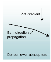
Decreasing index of refraction will typically cause path bending from transmitter to receiver, (towards the ground). That radius of curvature depends on n (or N), its gradient, and the angle of the path with respect to the horizon (α); it is approximated by:
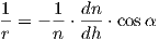 | (5.12) |
It is sometimes convenient to relate that curvature to a flat-earth model. We then define the effective radius of curvature over the radius of earth.
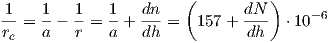 | (5.13) |
Microwave link designs often make use of a geoclimatic factor: K to indicate the amount of path bending. K is defined as the ratio of the effective ray bending over the radius of earth: K = re∕a.
Although it may not be required to know the radio index of refraction accurately for a given link, it is important to know if (when) that index changes significantly as it may alter the propagation path. General variation of N are around -40 per kilometer elevation, and so a commonly accepted average value for average normal atmospheric conditions is K=4/3.
These variations of the radio refractive index and K have several important impacts:
Copyright ©2018 Thomas Schwengler.
Even in clear conditions, temperature and water content variations may create refractive layers in the atmosphere, which impact microwave links exceeding several miles. These changes impact actual propagation paths, and therefore may cause severe multipath fading (when paths variations combine paths destructively). Scintillation fading due to smaller scale turbulent irregularities in the atmosphere may also have an impact at frequencies above about 40GHz. ITU-R recommendation P.530 [95] provides methods for predicting fading distributions at large fade depths in the average worst month.
Step 1: For the path location in question, estimate the geoclimatic factor K for the average worst month from fading data for the geographic area of interest. Formulas exist to approximate K, that depend on the area terrain roughness and dN1, the point refractivity gradient in the lowest 65m of the atmosphere not exceeded for 1% of an average year. dN1 is provided for instance on global maps in Recommendation ITU-R P.453. An estimate of K for planning purpose may be obtained from:
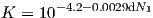 | (5.14) |
Step 2: From the transmitting and receiving antenna heights ht and hr (meters above sea level), calculate the magnitude of the path inclination |ϵp| (mrad) from |ϵp| = |hr - ht|∕d, where d is the path length (km). 4
Step 3: For detailed link design applications, calculate the percentage of time pw that fade depth A (dB) is exceeded in the average worst month; for small percentage of the time (around 0.01%):
 | (5.15) |
where f is the frequency (GHz), hL is the altitude of the lower antenna (the smaller of ht and hr), and K is the geoclimatic factor estimated above. (The overall standard deviation of error in predicting these fade margins are around 6dB).
The above number can be converted from a worst month percentage to an average yearly percentage by the formula:
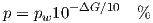 | (5.16) |
where
 | (5.17) |
where ΔG ≤ 10.8dB, d is the path length (km), L is the latitude (degrees N or S), |ϵp| is the path inclination (mrad), and the sign (±) in the equation is positive for latitudes below 45 degrees, and negative for latitude above 45 degrees.
Atmospheric absorption are dominated by water vapor and oxygen. Their atmospheric attenuation is given in a simple but good model for atmospheric gas attenuation in ITU-R report ITU-R P.676-6 “Attenuation by Atmospheric Gases” [97].
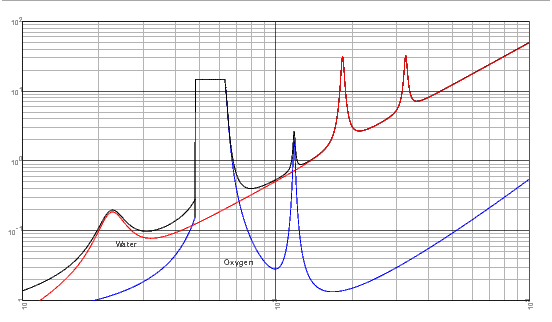
The water vapor absorption wary with humidity, and the absorption rate is estimated in dB/km by the formula below, as a function of the water vapor density (ρ in g/m3). At sea level, in continental climates (like Europe and continental US) a typical value ρ = 7.5g/m3 is often used.
 | (5.18) |
Attenuation peaks occur at frequencies of resonance of the water molecule (such as 23GHz, 183GHz, and 324GHz) where a lot of transmitted energy is absorbed and does not propagate very far.
The oxygen absorption is less variable and shows similar peaks of absorption at 60GHz and 120GHz. Its absorption rate in dB/km is defined piecewise as:
 | (5.19) |
The above formulas show that atmospheric attenuations and variations are minimal at frequencies below say 6GHz, and are rarely a consideration for cellular systems. Atmospheric absorptions (as well as rain fades) are however significant at higher frequencies, for which wireless links need to take into account the impact of this variability.
In addition to gaseous absorption, hydrometeors are also a severe cause of loss for frequencies above 10GHz or so. Heavy rain and especially large drop sizes have a severe impact. At 30GHz for instance heavy 50-100mm/hr precipitation causes 10-20dB/km attenuation, and will usually cause radio outages. This may be the case for LMDS (28-31GHz) or point-to-point microwave links (6, 11, 18, 23GHz).
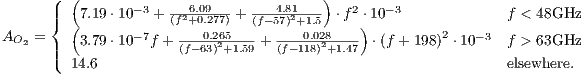
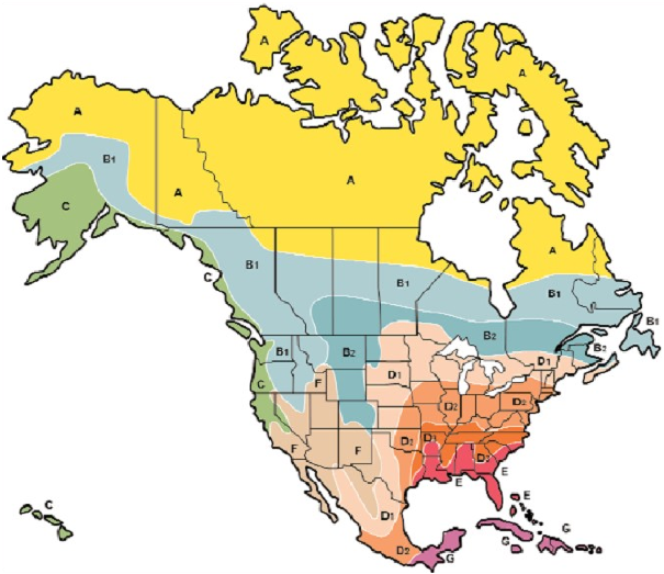
Water is a very lossy medium, and large rain drop sizes cause significant scattering, depolarization, and attenuation. As drop size increases, drops of rain tend to leave their nearly spherical shape, towards an oblate ellipsoid, which tends to affect vertical polarized wave less than horizontally polarized waves. Consequently, given the choice, microwave engineers prefer to use vertical polarization. Practically, however, measuring rain drop size is fairly difficult, and instead one has to rely on empirical average precipitation rates. Precipitation rates and probability of occurrence have been measured globally, and summarized in several rain regions.
Copyright ©2018 Thomas Schwengler.
Commonly used rain regions are either the ITU [99] or the Crane rain regions [101]; these region contours are used in order to gauge the probability of heavy rain outages. And maximum link distances are calculated for a certain percentage of availability. ITU recommendations have evolved with years, and include rain region contour very similar to the Crane regions, as well as statistical rain rate contours (in mm rain per hour) that are exceeded for 0.01% of the time in an average year.
Rainstorms tend to cluster into very localized phenomena, which typically only affect a portion of a radio link; consequently, an effective path length is defined to represent the distance (in km) attenuated by rain:
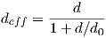 | (5.20) |
where d0 = 35e-0.015R0.01 (in km), and R0.01 is the rain rate (in mm per hour) exceeded in the region for 0.01% of the time (for R0.01 > 100mm/h, use R0.01 = 100mm/h). Rain intensity is given in the probability it exceeds a certain rate in table 5.1. Over this effective distance, for the precipitation rate occurring 0.01% of the time, rain attenuation (in dB) is estimated by:
 | (5.21) |
where k and α are coefficients given in table 5.2; they vary with frequency and polarization.
| %time | A | B | C | D | E | F | G | H | J | K | L | M | N | P | Q |
| 1.0 | < .1 | 0.5 | 0.7 | 2.1 | 0.6 | 1.7 | 3 | 2 | 8 | 1.5 | 2 | 4 | 5 | 12 | 24 |
| 0.3 | .8 | 2 | 2.8 | 4.5 | 2.4 | 4.5 | 7 | 4 | 13 | 4.2 | 7 | 11 | 15 | 34 | 49 |
| 0.1 | 2 | 3 | 5 | 8 | 6 | 8 | 12 | 10 | 20 | 12 | 15 | 22 | 35 | 65 | 72 |
| 0.03 | 5 | 6 | 9 | 13 | 12 | 15 | 20 | 18 | 28 | 23 | 33 | 40 | 65 | 105 | 96 |
| 0.01 | 8 | 12 | 15 | 19 | 22 | 28 | 30 | 32 | 35 | 42 | 60 | 63 | 95 | 145 | 115 |
| 0.003 | 14 | 21 | 26 | 29 | 41 | 54 | 45 | 55 | 45 | 70 | 105 | 95 | 140 | 200 | 142 |
| 0.001 | 22 | 32 | 42 | 42 | 70 | 78 | 65 | 83 | 55 | 100 | 150 | 120 | 180 | 250 | 170 |
Frequency (GHz) | kh | kv | αh | αv |
1 | 0.0000387 | 0.0000352 | 0.912 | 0.880 |
2 | 0.0001540 | 0.0001380 | 0.963 | 0.923 |
4 | 0.0006500 | 0.0005910 | 1.121 | 1.075 |
6 | 0.0017500 | 0.0015500 | 1.308 | 1.265 |
7 | 0.0030100 | 0.0026500 | 1.332 | 1.312 |
8 | 0.0045400 | 0.0039500 | 1.327 | 1.310 |
10 | 0.0101000 | 0.0088700 | 1.276 | 1.264 |
12 | 0.0188000 | 0.0168000 | 1.217 | 1.200 |
15 | 0.0367000 | 0.0335000 | 1.154 | 1.128 |
20 | 0.0751 | 0.0691 | 1.099 | 1.065 |
25 | 0.124 | 0.113 | 1.061 | 1.030 |
30 | 0.187 | 0.167 | 1.021 | 1.000 |
35 | 0.263 | 0.233 | 0.979 | 0.963 |
40 | 0.350 | 0.310 | 0.939 | 0.929 |
The above section gives a method to estimate rain attenuation (fade) 0.01% of the time in a given region. We may have other requirements for a radio links, which may need to evaluate attenuation corresponding to another percentage of link outage (for instance 0.1%, or more stringent 0.001%). In these cases we use a formula relating attenuation for a given percentage of the time Ap to attenuation A0.01 derived earlier in equation (5.21). [95]
| Percentage time p | Ap∕A0.01 | Ap∕A0.01 |
| (in %) | for lat<30o | for lat≥30o |
| 1 | 0.07 | 0.12 |
| 0.1 | 0.36 | 0.39 |
| 0.01 | 1 | 1 |
| 0.001 | 1.44 | 2.14 |
| formula for any p | 0.07 p-(0.855+0.139 log p) | 0.12 p-(0.546+0.043 log p) |
Effects of snow and ice tend to be less severe as those of rain. An experimental model [103] estimates attenuations at 0∘C (in dB/km): 5
 | (5.22) |
where R is the snowfall rate (in mm/hr of melted water content), λ is the wavelength (in cm). Typical snow falls yield attenuations of 0.2 to 1 dB/km, thus much lower than rain attenuations.
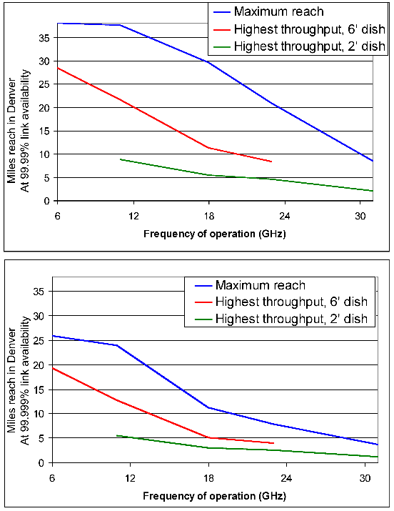
Of course microwave reach varies with: power, frequency, antenna size and gain (dish diameter 1 to 6 or even 8 feet), modulation & therefore throughput, rain region and availability (mostly impacted by rain outages). These variations and indicative distances can be summarized an in figure 5.10.
Millimeter waves usually refer to signals around 30 GHz to 300 GHz (or wavelengths from 1 to 10 mm). Millimeter wave links are used for point to point links under part 15 and part 101 rules in the US. They have the advantage of offering higher capacity (in excess of Gbps) but the disadvantage of being more attenuated by atmospheric effects.
Until recently, they have only been considered for line of sight links because of their high diffraction loss, but recent efforts to increase wireless links further is now showing renewed interest at higher frequencies for short non-line-of-sight high-capacity applications. The advantage of millimeter waves are their small wavelength, hence the smaller antenna size, hence the great potential for MIMO and massive MIMO applications with many antennas (up to 64 today, hundreds or even thousands are in R&D phases).
Some bands are already active: 60GHz unlicensed with point to point and WirelessHD, IEEE 802.11ad, and IEEE 802.15.3c; 70-80-90GHz eBand are used as well. Recent initiatives are pushing to open more bands [28]:
Calculate
Copyright ©2019 Thomas Schwengler. A significantly updated and completed 2019 Edition is available.