9 MIMO

Support independent publishing: Buy this book on Lulu.

Chapter 9
MIMO

This chapter is an introduction to Multiple Input Multiple Output radio systems. It presents the underlying fundamentals of MIMO, with some theoretical aspects as well as some practical applications in modern wireless standards making use of MIMO.

Significantly updated and completed in 2019 Edition available here.

9.1 Introduction

MIMO techniques are the most important advance in recent wireless systems; they are a critical part of important standards such as LTE (and LTE Advanced), HSPA+, WiMax, 802.20, 802.11n/ac/ad The purpose of MIMO is mainly to increase throughput (with multiple streams). MIMO systems are also used to increase reach and lower interference (with beam forming), and to improve data integrity (with coding, preconditioning, diversity).

9.1.1 History

Bell Labs research started research on MIMO in the 80’s, but one of the turning point might have been the major attention given by the media to BLAST, the Bell Labs Space Time which demonstrated impressive throughput rates.

9.1.2 Techniques

At least five multi-antenna techniques are used to improve link performance:

Receive diversity : classic selection, MRC, the method has been used at the base station since the early days of cellular telephony. Of course the concept of combining multiple receivers to fight fading is even older, and widely used such as in microwave links. More recently it is seeing renewed interest on a smaller scale in multiple antennas in mobile handsets.
Transmit diversity using Space-Frequency Block Coding (SFBC) at the base station.
Beam Steering (towards a specific device) and null forming (for interference cancellation). This is the classic approach for an antenna array designer.
MIMO spatial multiplexing at the base station, for multiple user access.
Cyclic Delay Diversity (CDD), used with spatial multiplexing (an OFDM technique).

9.1.3 Capacity

The main theoretical aspect of MIMO is one of channel capacity. The Shanon’s capacity theorem for a simple RF channel is:

C = B log (1 + S∕N ) 2

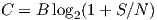(9.1)

where C= capacity (bits/s), B=bandwidth (Hz), S∕N= signal to noise ratio.

That capacity equation ¹ is widely used and refers to a system with one transmitter, and one receiver (with possibly added diversity, but ultimately combined into one receiver); now we consider a system of N × M antennas: N transmitters, and M receivers.

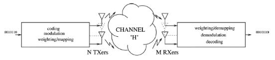
Figure 9.1: MIMO channel is represented by a N×M matrix of throughput correlation parameters (amplitude and phase) from each transmitted signal to each received signal.

The H-matrix is a matrix [H_ij] defines complex throughput correlation parameters (with amplitude and phase) from each transmit antenna i to each receive antenna j. The new capacity equation for MIMO systems is

∑n ( ) C = B log2 1 + Siσ2i(H ) i=1 N

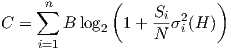(9.2)

where n is the number of independent transmit/receive channels (which is no greater than min(N,M)), and reflects the number of sufficiently uncorrelated paths (It is the rank of the matrix H, and in LTE it is referred to as the rank of the channel), S_i are the signal power in channel i, N the noise power, and σ_i²(H) are singular values of the H matrix.

This channel capacity equation shows that capacity increases linearly with n, which optimally approaches the number of antennas min(N,M). But remember that the channel itself (meaning the propagation media) has a rank, and has a capacity, no matter how many antennas are in the system.

That linear variation is where the value of MIMO lies. In equation (9.1), capacity increases in log ₂(1+SNR), which is nearly a linear increase in SNR for small values of SNR (since log(1+x) ≈ x for x ≈ 0), however modern wireless standards tend to aim at higher modulation rates, which require higher SNR, for which log ₂(1+SNR) ≈ log ₂(SNR), which is a much slower increase in capacity.

9.2 Fundamental Principles

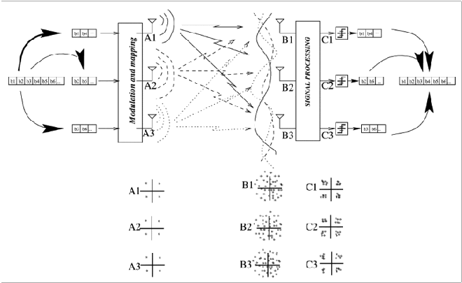
MIMO systems include considerations around signal preconditioning, as well as channel predictions, as illustrated in figure 9.2.

Figure 9.2: This great diagram (from [152]) illustrates preconditioning, channel variations, and processing. Each transmit signal is mapped into layers (streams), which are sent on each antenna. The receiving side retrieves the initial signal from the multiple received layers.

For the complete chapter, please see the 2019 edition available here.